Simulated Maximum Likelihood with PFJAX
Pranav Subramani, Mohan Wu, Martin Lysy – University of Waterloo
September 13, 2022
Summary
In the Introduction to PFJAX, we saw how to set up a model class for a state-space model and how to use a particle filter to estimate its marginal loglikelihood \(\ell(\tth) = \log p(\yy_{0:T} \mid \tth)\). In this tutorial, we’ll use PFJAX to approximate the maximum likelihood estimator \(\hat \tth = \argmax_{\tth} \ell(\tth)\) and its variance \(\var(\hat \tth)\).
Benchmark Model
We’ll be using a Bootstrap filter for the Brownian motion with drift model defined in the Introduction:
where the model parameters are \(\tth = (\mu, \sigma, \tau)\). The details of setting up the appropriate model class are provided in the Introduction. Here we’ll use the version of this model provided with PFJAX: pfjax.models.BMModel.
# jax
import jax
import jax.numpy as jnp
import jax.scipy as jsp
import jax.random
from functools import partial
# plotting
import numpy as np
import pandas as pd
import seaborn as sns
import matplotlib.pyplot as plt
import projplot as pjp
# pfjax
import pfjax as pf
from pfjax.models import BMModel
# stochastic optimization
import optax
WARNING:jax._src.lib.xla_bridge:No GPU/TPU found, falling back to CPU. (Set TF_CPP_MIN_LOG_LEVEL=0 and rerun for more info.)
Simulate Data
# parameter values
mu = 0.
sigma = .2
tau = .1
theta_true = jnp.array([mu, sigma, tau])
# data specification
dt = .5
n_obs = 100
x_init = jnp.array(0.)
# initial key for random numbers
key = jax.random.PRNGKey(0)
# simulate data
bm_model = BMModel(dt=dt)
key, subkey = jax.random.split(key)
y_meas, x_state = pf.simulate(
model=bm_model,
key=subkey,
n_obs=n_obs,
x_init=x_init,
theta=theta_true
)
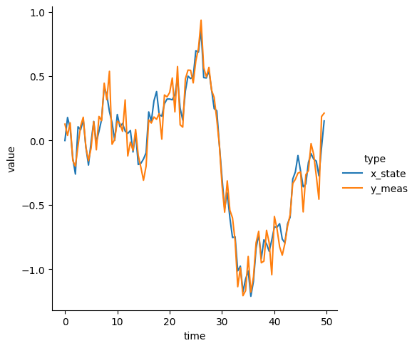
# plot data
plot_df = (pd.DataFrame({"time": jnp.arange(n_obs) * dt,
"x_state": jnp.squeeze(x_state),
"y_meas": jnp.squeeze(y_meas)})
.melt(id_vars="time", var_name="type"))
sns.relplot(
data=plot_df, kind="line",
x="time", y="value", hue="type"
)
<seaborn.axisgrid.FacetGrid at 0x7fbc4f2cc990>
Stochastic Optimization
The first step to performing simulated maximum likelihood estimation with PFJAX is to estimate the MLE \(\hat \tth = \argmax_{\tth} \ell(\tth)\). To do this, we perform stochastic optimization of the particle filter objective function \(\hat{\ell}(\tth)\), for which we’ll need to approximate the score function \(\nabla \ell(\tth) = \frac{\partial}{\partial \tth} \ell(\tth)\).
A straightforward approximation would be to use JAX to directly differentiate the particle filter approximation \(\hat{\ell}(\tth)\). However, this turns out to be biased [2], in that in general \(E[\frac{\partial}{\partial \tth} \hat{\ell}(\tth)] \neq \frac{\partial}{\partial \tth} \ell(\tth)\). The Gradient Comparisons notebook compares the speed and accuracy of several stochastic approximations to the score function. The recommended algorithm [5] is implemented in pfjax.particle_filter_rb(). Note that this algorithm scales quadratically in the number of particles, whereas scaling is only linear with the basic particle filter pfjax.particle_filter(). However, the quadratic algorithm requires far fewer particles for comparable (but superior) accuracy and speed.
We’ll use the Optax package for gradient-based stochastic optimization in the code below. First we write a simple wrapper function to stochastically maximize PFJAX state-space models.
def pf_stochopt(model, key, theta, y_meas, n_particles,
                learning_rate, n_steps):
    """
    Stochastic optimization using Adam.

    Args:
        model: A particle filter model object.
        key: PRNG key.
        theta: Initial parameter value.
        y_meas: JAX array with leading dimension `n_obs` containing the measurement variables
                `y_meas = (y_0, ..., y_T)`, where `T = n_obs-1`.
        n_particles: The number of particles to use in the particle filter.
        learning_rate: Optimizer learning rate.
        n_steps: Number of optimizer steps.

    Returns:
        theta: Parameter value at last step.
        loglik: JAX array of length `n_steps` containing a stochastic estimate of the loglikelihood at each step.
    """
    # set up and initialize the optimizer
    optimizer = optax.adam(learning_rate=learning_rate)
    opt_state = optimizer.init(params=theta)

    # optimizer step function
    @jax.jit
    def step(theta, key, opt_state):
        pf_out = pf.particle_filter_rb(
            model=model,
            key=key,
            y_meas=y_meas,
            n_particles=n_particles,
            theta=theta,
            history=False,
            score=True,
            fisher=False
        )
        opt_updates, opt_state = optimizer.update(
            updates=-1.0 * pf_out["score"], # optax assumes a minimization problem
            state=opt_state,
            params=theta
        )
        theta = optax.apply_updates(params=theta, updates=opt_updates)
        return theta, opt_state, pf_out["loglik"]

    # optimizer loop
    subkeys = jax.random.split(key, n_steps)
    loglik_out = jnp.zeros((n_steps,))
    for i in jnp.arange(n_steps):
        theta, opt_state, loglik = step(theta=theta, key=subkeys[i], opt_state=opt_state)
        loglik_out = loglik_out.at[i].set(loglik)

    return theta, loglik_out
Next, we perform stochastic optimization for the Brownian motion model and the simulated data.
# optimization setup
theta_init = jnp.array([1., 1., 1.])
n_particles = 50
learning_rate = 0.01
n_steps = 200

theta_opt, loglik = pf_stochopt(
    model=bm_model,
    key=key,
    theta=theta_init,
    y_meas=y_meas,
    n_particles=n_particles,
    learning_rate=learning_rate,
    n_steps=n_steps
)

# plot loglikelihood as a function of step count
sns.relplot(
    data = {"step": jnp.arange(n_steps), "loglik": loglik},
    x = "step",
    y = "loglik"
)

# estimated and true parameter values
{"theta_opt": jnp.round(theta_opt, decimals=2), "theta_true": theta_true}
{'theta_opt': DeviceArray([0.  , 0.19, 0.12], dtype=float32),
 'theta_true': DeviceArray([0. , 0.2, 0.1], dtype=float32)}
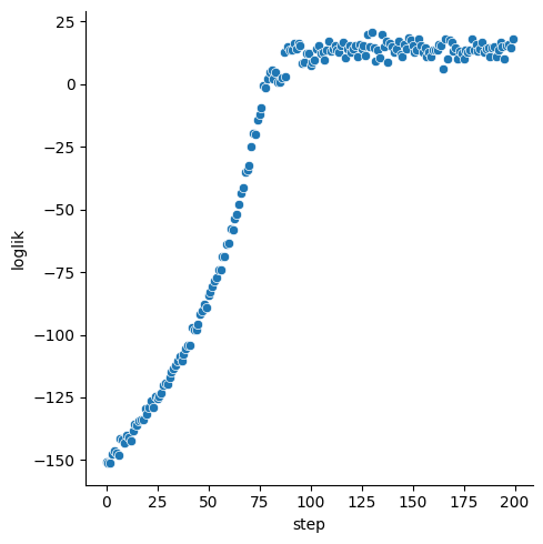
We see that the stochastic optimization converged after about 100 steps and that the estimate \(\hat \tth\) is very close to the true parameter value.
Variance Estimation
Suppose we had the MLE of the exact marginal likelihood, \(\tilde{\tth} = \argmax_{\tth} \ell(\tth)\). Then the standard method of estimating its variance \(\var(\tilde{\tth})\) is by taking the inverse of the observed Fisher information,
Therefore, a natural choice of variance estimator for the stochastic maximum likelihood estimate \(\hat{\tth}\) calculated above is the inverse of the expected value of the observed Fisher information taken over the particles,
Once again, we use the algorithm of Poyiadjis et al. [5] to obtain a consistent estimate of the expectation above, and calculate the variance estimator in the code below.
@partial(jax.jit, static_argnums=(0, 4))
def pf_varest(model, key, theta, y_meas, n_particles):
    """
    Variance estimation for stochastic optimization.

    Args:
        model: A particle filter model object.
        key: PRNG key.
        theta: Initial parameter value.
        y_meas: JAX array with leading dimension `n_obs` containing the measurement variables
                `y_meas = (y_0, ..., y_T)`, where `T = n_obs-1`.
        n_particles: The number of particles to use in the particle filter.

    Returns:
        varest: Variance estimate.
    """

    pf_out = pf.particle_filter_rb(
        model=model,
        key=key,
        y_meas=y_meas,
        n_particles=n_particles,
        theta=theta,
        history=False,
        score=True,
        fisher=True
    )
    return jnp.linalg.inv(pf_out["fisher"])

# calculate the variance estimate
n_particles = 100 # increase this a bit since the calculation only needs to be done once

theta_ve = pf_varest(
    model=bm_model,
    key=key,
    theta=theta_opt,
    y_meas=y_meas,
    n_particles=n_particles
)

theta_ve
DeviceArray([[ 7.4947055e-04,  3.5483090e-06, -5.5172131e-06],
             [ 3.5483247e-06,  7.4144156e-04, -3.0139703e-04],
             [-5.5172195e-06, -3.0139703e-04,  4.0273910e-04]],            dtype=float32)
Finally, we should check that the variance estimator is positive definite.
np.linalg.eigvalsh(theta_ve)
array([0.00022636, 0.00074928, 0.00091801], dtype=float32)